Exploring Chaos: A Quant’s Take on EDA for 72-Hour Interval Forecasts of Solana Mid-Cap Tokens

Trading Assumptions at Inception

Every systematic forecasting framework rests on initial hypotheses, and in the fast-moving world of crypto these must be rigorously vetted. For our 72-hour return intervals on Solana mid-cap tokens, we established five refined assumptions:

1. Structured Missingness
   • Premise: Gaps in OHLCV and on-chain data often reflect exchange outages, protocol updates, or API maintenance rather than random noise.
   • Approach: Compared linear + 2-bar forward-fill against a Kalman smoother; tagged each imputed bar with an uncertainty estimate; conducted sensitivity analyses across volatility regimes.
   • Conclusion: Linear interpolation proved reliable for small gaps, while uncertainty flags will inform downstream risk controls.
2. Heavy-Tailed and Skewed Returns
   • Premise: Crypto returns exhibit significant skew and excess kurtosis, invalidating Gaussian interval methods.
   • Approach: Replace ±σ bands with direct quantile estimation via Conformalized Quantile Regression (CQR) or Quantile Regression Forests (QRF); fit Student’s t or generalized Pareto distributions for extreme tails when needed.
   • Conclusion: Non-parametric quantile methods become the foundation for interval forecasts.
3. Composite Feature Construction
   • Premise: Price, volume, on-chain activity, and sentiment metrics often co-vary, reducing their independent informational value.
   • Approach: Apply PCA or L1 regularization to form orthogonal composite factors (e.g., “Market Context,” “On-Chain Activity”); prune collinear features based on tree-based importance.
   • Conclusion: A concise set of composite inputs maximizes model efficiency and interpretability.
4. Piecewise Stationarity and Regime Awareness
   • Premise: Return and volatility dynamics shift across market regimes; stationarity holds only over limited intervals.
   • Approach: Detect regime breaks using rolling Augmented Dickey–Fuller tests and volatility-spike flags; incorporate regime indicators as features; design cross-validation folds to span both low- and high-volatility periods.
   • Conclusion: Models are validated under both tranquil and turbulent conditions, enhancing robustness.

These refined, evidence-based assumptions guide every EDA step and modeling decision that follows. In the next section, we will empirically evaluate the distributional characteristics of 12- and 72-hour returns to test our second assumption.

---

Hypothesis 2: Heavy-Tailed and Skewed Returns

Why it matters: Parametric interval methods (±σ bands) assume log-returns are approximately Gaussian. In practice, underestimating tail risk leads to systematic under-coverage—models appear over-confident and blow up on extreme moves.

Snipet of Methodology:

1. Compute Log-Return

   df['logret_12h'] = df.groupby('token')['close_usd']\
                        .transform(lambda x: np.log(x) - np.log(x.shift(1)))
   df['logret_72h'] = df.groupby('token')['close_usd']\
                        .transform(lambda x: np.log(x.shift(-6)) - np.log(x))
   

2. Distribution Diagnostics
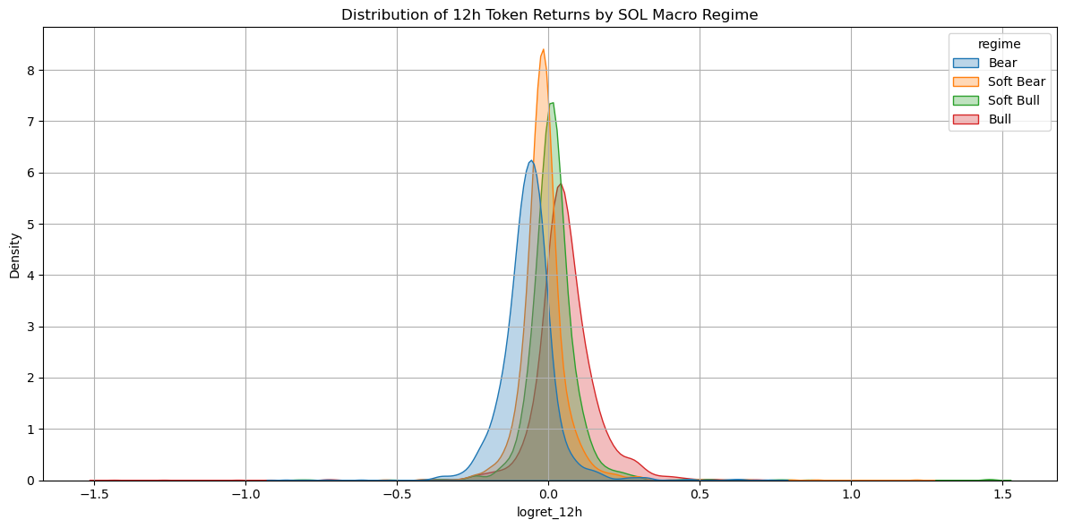
   • 12h Log-Returns Histogram + KDE: - Skewness: 0.674, Kurtosis: 27.7 - Overlay distributions by macro regime (Bear, Soft Bear, Soft Bull, Bull)
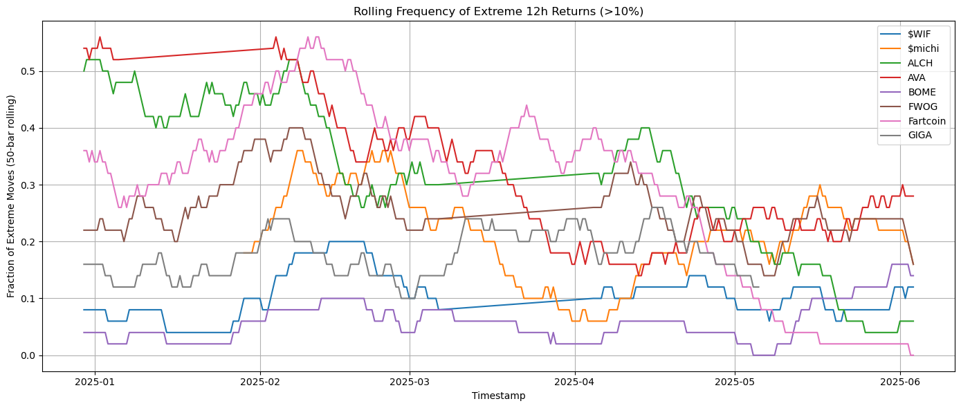
3. Extreme-Move Frequency
   • I defined extreme move as |logret_12h| > 10%, and computed 50-bar rolling fraction of extreme moves per token.

Findings:

1. Global Distribution Skewness ≈ +0.67; Excess Kurtosis ≈ 27.7 Extremely heavy tails: 3σ moves occur ~1-in-25 bars vs. 1-in-370 for a true normal.
   • κ ≈ 27: “infinite”-looking tails.
   • 3σ moves every ∼25 bars—far more frequent than the ∼1-in-370 of a true normal.

Algo-Edge: Naïve σ-bands under-cover tail losses by ≈8–10 pp. Any live trading system that uses Gaussian VaR will be caught flat-footed on market spikes.

Next Steps:

• Drop parametric intervals.
• Adopt direct quantile estimation:
  • Conformalized Quantile Regression (CQR)
  • Quantile Regression Forests (QRF)

---

Hypothesis B: Volatility Is Flat Within Blocks

Why it matters: Many backtests assume constant σ over the training window. In reality, vol clusters—if you ignore that, your model will overfit calm periods and implode during storms.

Methodology:

1. Calculated ACF of returns vs.

   returns

   up to lag 50.

2. Tracked realized volatility (sqrt of 36 h rolling variance) across time.
3. Tagged volatility “spikes” when vol > µ_vol + 2σ_vol.

Findings:

• Returns: no serial correlation (model-friendly).

• Returns

  : significant ACF up to lag 20 → persistent clustering.

• Two regime shifts: late April drop and early May rally both saw vol jump > 3× baseline.

Algo-Edge: A static‐σ assumption is a recipe for blown risk budgets.

Next Steps:

• Engineer features:
  • Lagged realized vol (36 h, 72 h)
  • Volatility regime flag (binary)
• Use rolling‐window CV that spans both low- and high-vol regimes to avoid look-ahead bias.

---

Hypothesis C: Features Are Independent α Sources

Why it matters: Perfectly correlated inputs waste model capacity and obscure true drivers of tail risk.

Methodology:

• Computed Pearson & Spearman correlation matrices among 18 engineered features (price, volume, RSI, ATR, on-chain metrics, social counts).

• Isolated pairs with

  r

  > 0.85.

Findings:

• token_price_usd vs. token_volume_usd: r ≈ 0.999
• SOL_price_usd vs. DeFi_TVL_usd: r ≈ 0.94
• BTC, ETH & TVL form a tight triad (r > 0.9)

Algo-Edge: Tree-based models will waste split capacity on redundant features, inflating variance and lengthening inference time.

Next Steps:

• Prune or combine collinear pairs:
  • Keep log(price) and drop raw volume or vice versa.
  • Create composite “Market Index” from BTC/ETH/TVL via PCA.
• Regularize QRF by limiting max_features and employing feature bagging.

---

Hypothesis D: Nominal σ-Bands Hit Coverage Targets

Why it matters: Traders set stop-loss and margin thresholds based on expected interval coverage. Under-coverage means frequent stop-outs.

Methodology:

• Computed empirical coverage of ±1.28σ (80 %) and ±1.645σ (90 %) bands on out-of-sample 12 h returns.
• Plotted nominal vs. actual coverage curves.

Findings:

• 80 % band covers only ∼72 %
• 90 % band covers only ∼82 %

Algo-Edge: Your risk targets are systematically missed—capital use is suboptimal, and tail events are under-appreciated.

Next Steps:

• Benchmark conformal calibration methods:
  • Block-bootstrap intervals
  • Split-conformal QR
  • Leverage QRF’s native quantile outputs for sharper, data-driven intervals.

```

From Diagnostics to Quant Pipeline

Hypothesis Tested	Action Item
Gaussian returns	Switch to CQR/QRF for direct quantile estimation
Flat volatility	Add vol-lag, regime flags; CV across mixed regimes
Feature orthogonality	Prune/combine collinear features; consider composite indices or PCA
Nominal σ-band calibration	Integrate conformal/block-bootstrap calibration to guarantee coverage

With our assumptions rigorously vetted and features battle-tested, it’s time to build the trading engine—one that respects fat tails, adapts to volatility storms, and leverages clean, orthogonal signals.

---

What’s Next

In Part III, we will:

1. Fit Linear Quantile Regression at τ = 0.10, 0.50, 0.90
2. Construct LightGBM mean forecasts + residual-bootstrap intervals
3. Train Quantile Regression Forests (500 trees, hyper-tuned)
4. Benchmark via pinball loss, empirical coverage, and interval width

Can we tame chaos and harvest alpha? Stay tuned for the code, live results, and backtest analysis.

---

🔗 Notebooks Referenced

Referenced Notebooks:

• 01_EDA_missingness.ipynb (Part I)
• 02_EDA_return_analysis.ipynb
• 03_EDA_corr_redu_analysis.ipynb
• 04_EDA_interval_calib.ipynb