Research Under Uncertainty: Why This Work Matters
Building a model is only half the battle. In volatile crypto markets, the quality of your dataset defines the ceiling of your forecasting potential.
My aim wasn’t just to build a dataset — it was to construct a research-grade panel that could support tail-sensitive, quantile-based forecasting and provide solid base to backtest additional trading strategies.
So before modelling, I focused on a harder problem: trusting the data. This post walks through how I constructed a clean, 12-hour-resolution panel for 23 mid-cap Solana tokens, merging price, liquidity, and on-chain behaviour - and ensuring every entry is traceable, aligned, and imputation-aware.
🧩 The Raw Inputs: 12-Hour Multi-Source Panel
I aggregated data from multiple APIs and tools into synchronized 12-hour windows. I didn’t just need OHLCV — I needed enough dimensionality to explain volatility spikes, tail risks, and asymmetric behaviours. That meant pulling in signals from on-chain metrics, market-wide flows, and Solana ecosystem activity.
Included Streams:
- OHLCV per token (SolanaTracker APIs)
- On-chain metrics:
holder_count,transfer_count,new_token_accounts(CoinGecko API) - Global crypto context: SOL, ETH, BTC prices; DeFi TVL; Solana network tx count; SPL instruction count (CoinGecko and Big Query Solana Community Public Dataset)
- Social Media Sentiment Datastream not included but was created (LunarCrush API)
📒 See notebook:
01_EDA_missingness.ipynb
🧹 Cleaning the OHLCV Panel
Tokens like $COLLAT and titcoin were removed due to excessive missingness or late data starts. All data was reindexed to a 12h frequency.
This wasn’t just a practical step, it was a research design choice. Tokens with late listings or erratic gaps could inject bias into quantile estimates, especially in the tails. I chose to cut aggressively, favouring consistency over sample size.
I then clipped each token’s history at the first valid OHLCV bar using this logic:
# Pseudocode: clip token history post-launch
token_start = df[~df[ohlcv_cols].isnull().any(axis=1)].groupby('token')['timestamp'].min()
df['post_launch'] = df.apply(lambda r: r['timestamp'] >= token_start.get(r['token'], r['timestamp']), axis=1)
df = df[df['post_launch']]
📒 See full notebook:
01data_processing.ipynb
🔎 Auditing the Damage: OHLCV Missingness
Before cleaning, OHLCV columns had ~18% missing values, due to missing data coverage in the Solana Tracker API — not timestamp issues.
This heatmap shows how gaps differ across tokens:
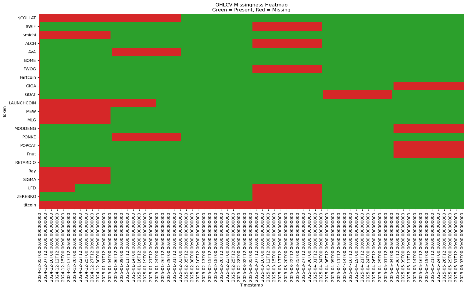
Green = present, Red = missing
Plot from notebook:
01_EDA_missingness.ipynb
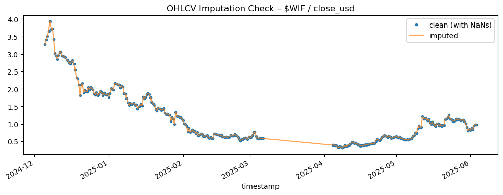
🔄 Imputation Strategy: Linear > Kalman
To fill the gaps, I benchmarked multiple methods: Kalman smoothing, PCA, k-NN, forward-fill, and linear interpolation — using simulated missingness and RMSE as the metric.
I initially considered Kalman smoothing and PCA-based methods — but rigorous testing with simulated gaps showed that linear interpolation actually outperformed them. This taught me something subtle: when your goal is to model distributional uncertainty, overly sophisticated imputation can backfire. Kalman filtering and PCA impose structure that might wash away useful volatility signals. Linear interpolation, though simple, preserved the noise that actually carries meaning in crypto returns.
# Comparison of imputation RMSE (5% simulated gaps)
methods = {
    'ffill_lim2': 0.09185,
    'linear_interp': 0.06042,
    'knn': 0.93970,
    'kalman': 0.09185
}
Conclusion: Linear interpolation + 2-bar forward-fill wins.
Full benchmarks in notebook:
03OHLCV_cleaning_imputation.ipynb
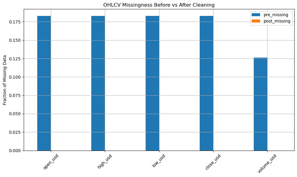
📊 Audit Results
After cleaning:
- Rows dropped: 22.36%
- Final rows: 6,464
- OHLCV missingness: 0%
- On-chain features missingness: reduced and tracked
I transformed a noisy, half-usable time series into a modeling-ready dataset — one where every token had a coherent timeline, every bar had traceable logic, and downstream features could be computed with confidence.
Bar chart from audit:
Example OHLCV Imputation for WIF Token:
More visuals and breakdowns in:
02cleaning_ohlcv_data.ipynb
Lessons Learned
If I had started modeling too early, I’d have baked in structural bias. Instead, by building a consistent data foundation, I now trust that any prediction error I see belongs to the model — not the data.
- 🔎 Token timelines matter: I built a
post_ohlcv_launchflag per token to avoid spurious early entries. - ⚖️ Linear interpolation can outperform complex models in practice — especially when gaps are small.
- 📉 Removing ~22% of rows may feel painful, but it’s necessary to preserve modeling integrity.
🧰 The Final Product
The master dataset — now stored as solana_cleaned_imputed_final.parquet includes:
- Fully cleaned OHLCV
- Timestamp-aligned token and market features
- Flags for imputed rows, clipped starts, and modeling-ready alignment
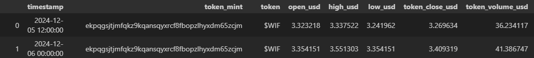
Example preview:
df_imputed.head()
🛤️ Coming Up Next…
In the next post, I’ll cover how I conducted exploratory analysis and some insights into the On-Chain lives of the tokens:
- Return Analysis and Correlation Reduction Analysis
- Interval Calibration and CQR/QRF Rolling Calibration
- Insights into Feature Engineering and Model Development